Bézier curves

Bézier curves are a popular classical approach for the purpose of freeform modelling. See wikipedia for a detailed explanation of those curves. I implemented the de Casteljau algorithm in order to evaluate such a curve. In the following are some screens taken from my tool (this application uses Swing):

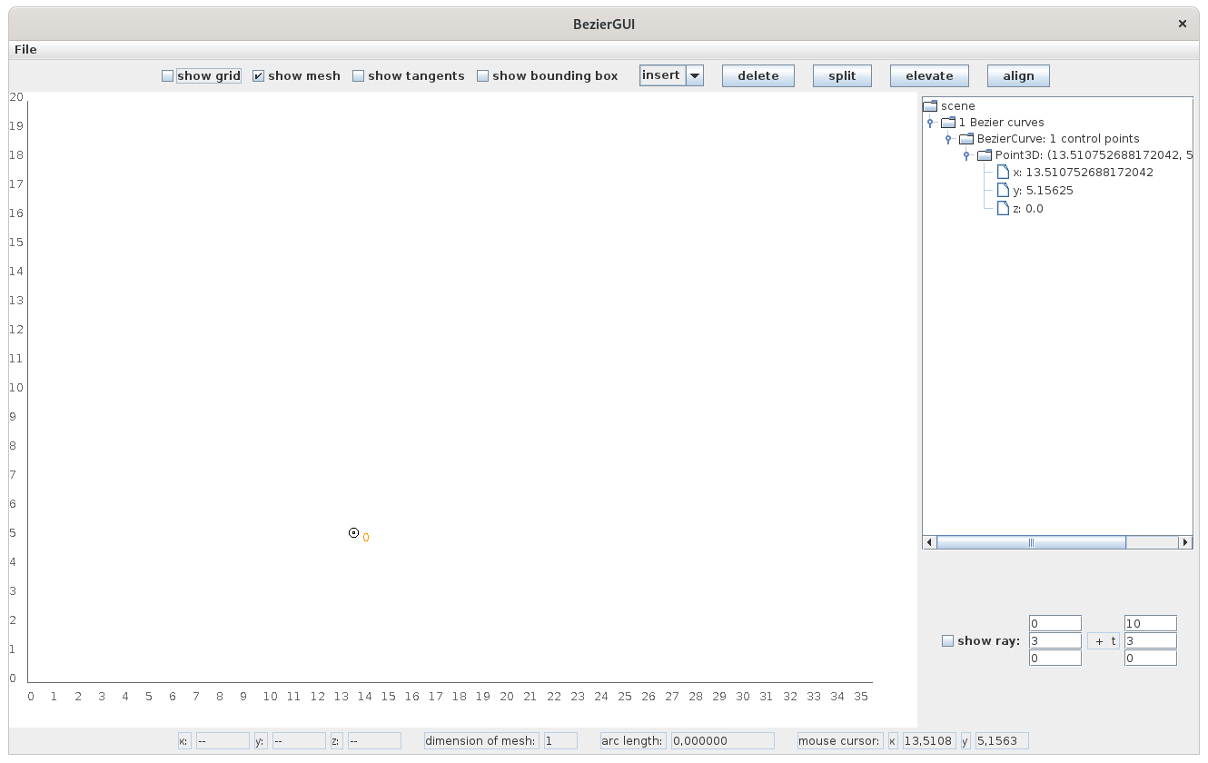
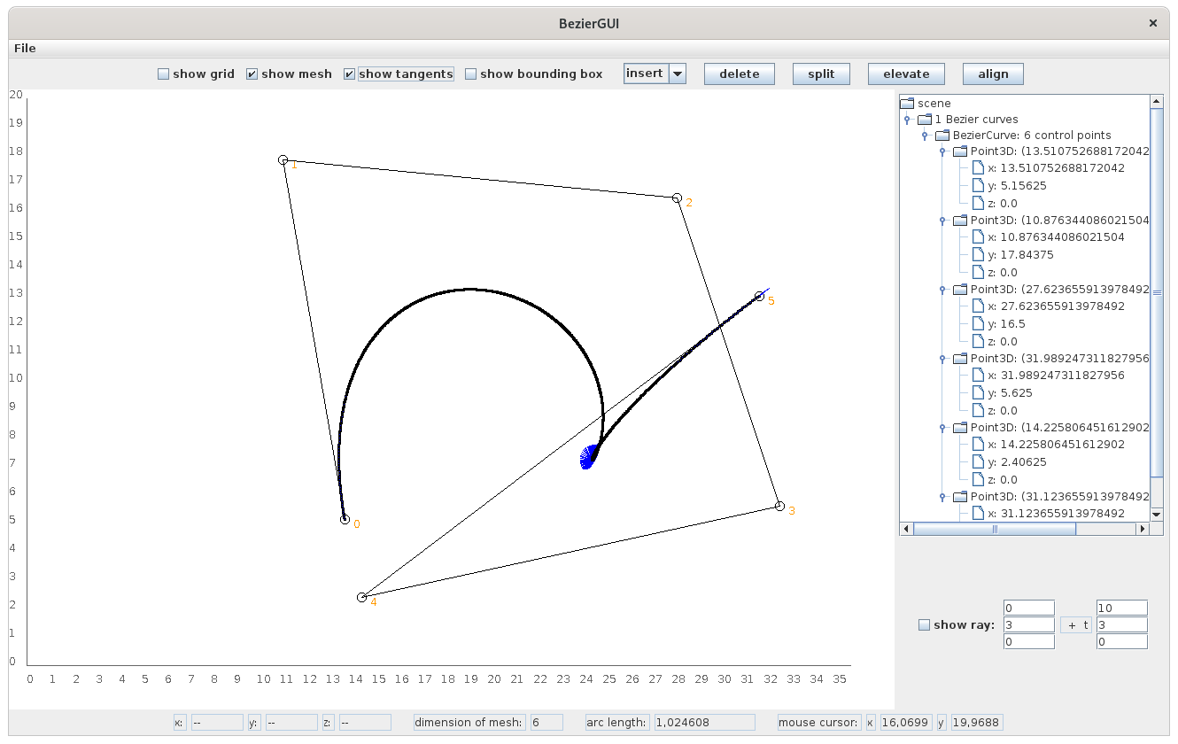
The screen above shows the application as it appears after it has been started. It consists of the main panel, where control points for a Bézier curve can be placed by simply clicking the left mouse button. Above this panel is a control panel providing several check boxes and buttons influencing the curve. Directly below the main panel is a status panel providing useful information about the curve under consideration, like, e.g., the coordinates of a selected control point, the total number of control points for the curve, and its arc length. At the right of the screen there is a scene graph giving an overview of the control points already defined previously. 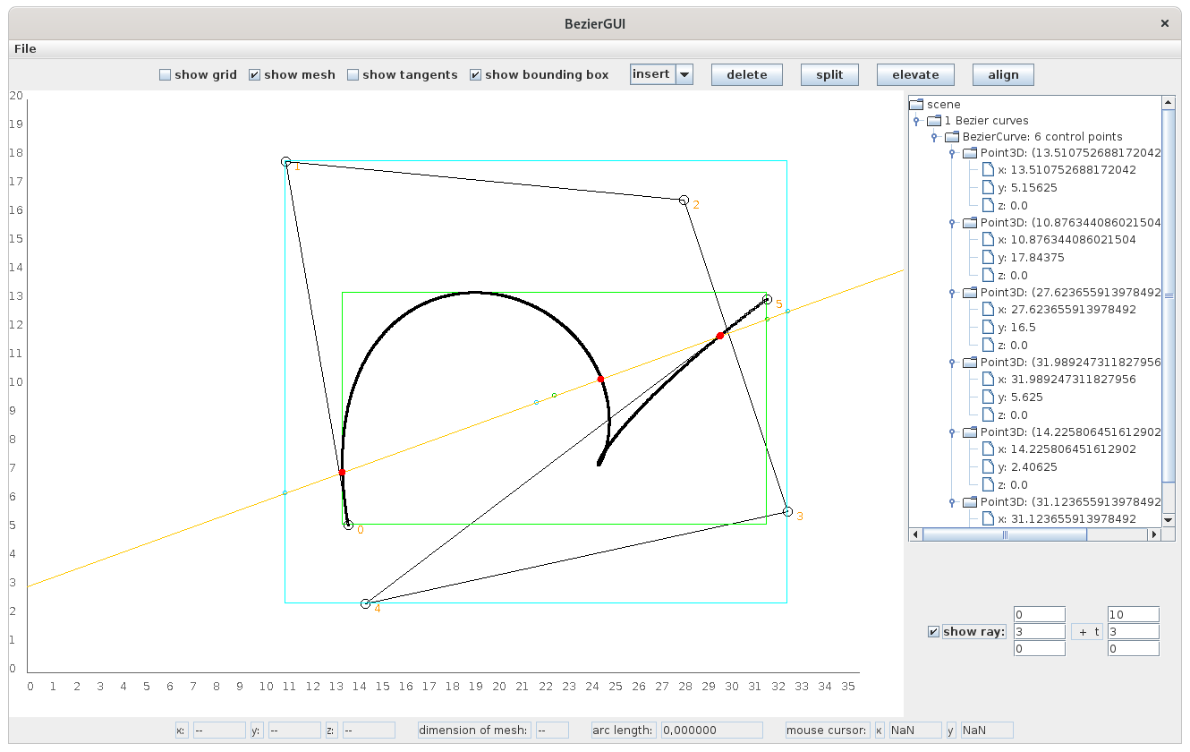Last but not least there exists a panel giving the possibility to draw a 3-dimensional ray within the scene in order to see the intersection points of the Bézier curves with this ray. Such a ray plays a crucial role when using ray tracing in order to render a scene (please pay attention to the next section).

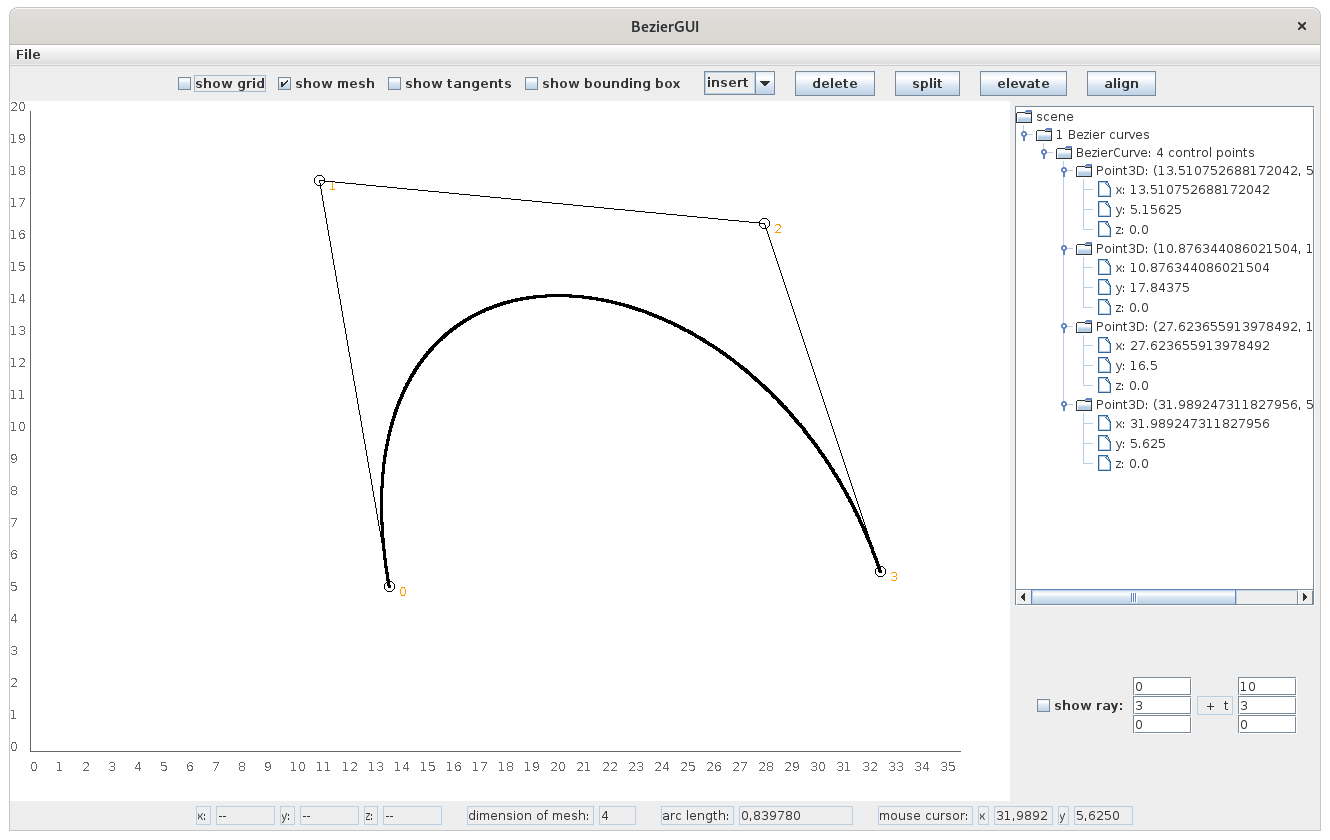
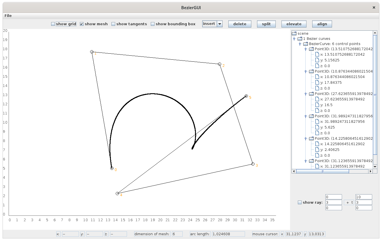
A Bézier curve will be defined by inserting control points to its control mesh. Each control point defined at the main panel will be reflected automatically by the scene overview on the right. Below, you can see how a Bézier curve will develop due to several mouse clicks:

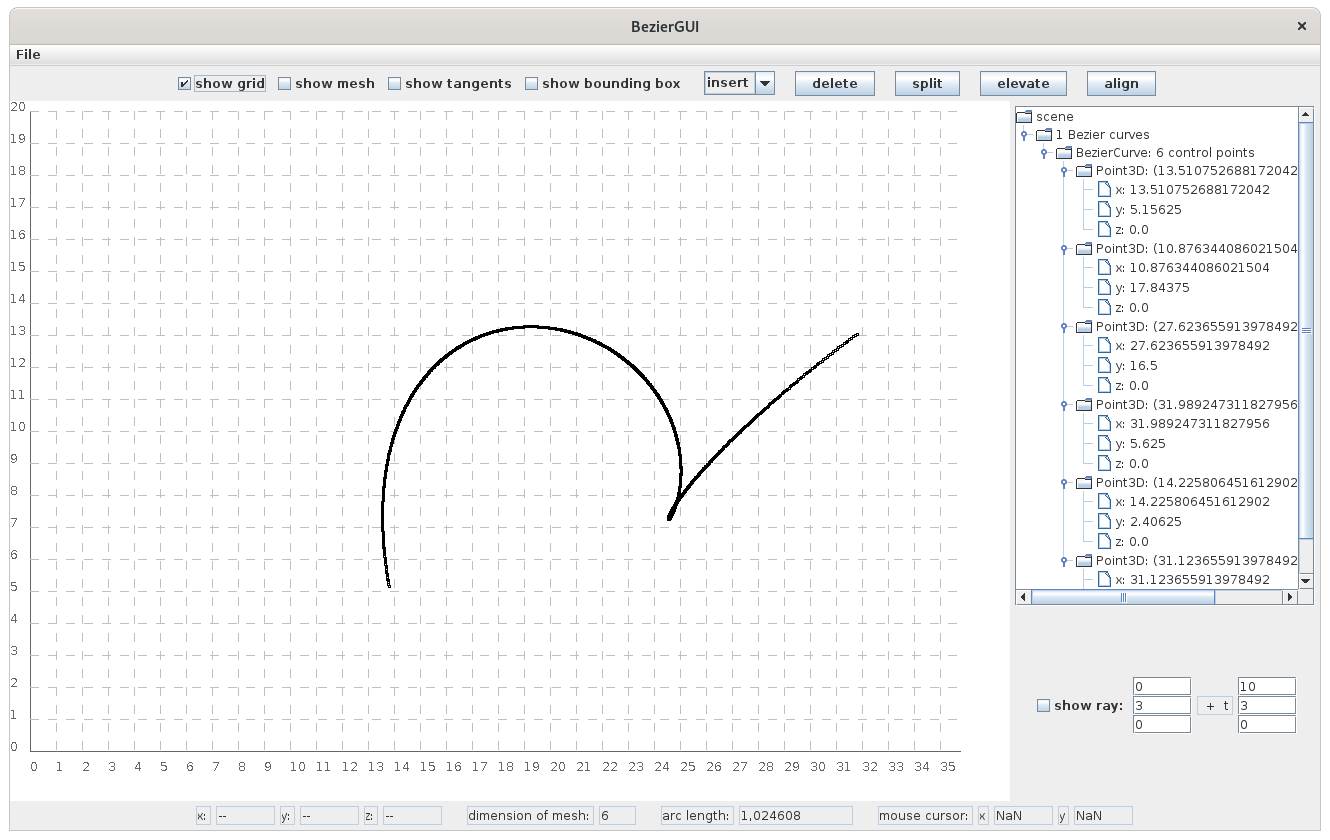
Here, you can see the final curve without its control points, but the grid of the coordinate system has been activated:

When one activates the check box show tangents the application draws blue lines representing the tangents at the corresponding evaluated points. Those tangents are for example useful for the computation of the normal at the corresponding point (one needs normals for rendering purposes).

The next screen shows the possibility to select a specific control point within the mesh. The selected control point is represented by a square surrounding it. The status panel gets refreshed automatically in order to show the coordinates of this control point. It is now possible to relocate the control point on the drawing canvas, or to simply delete it by using the button delete. This automatically triggers a new drawing of the resulting curve where the control point has been removed from the mesh (and as well from the overview on the right).

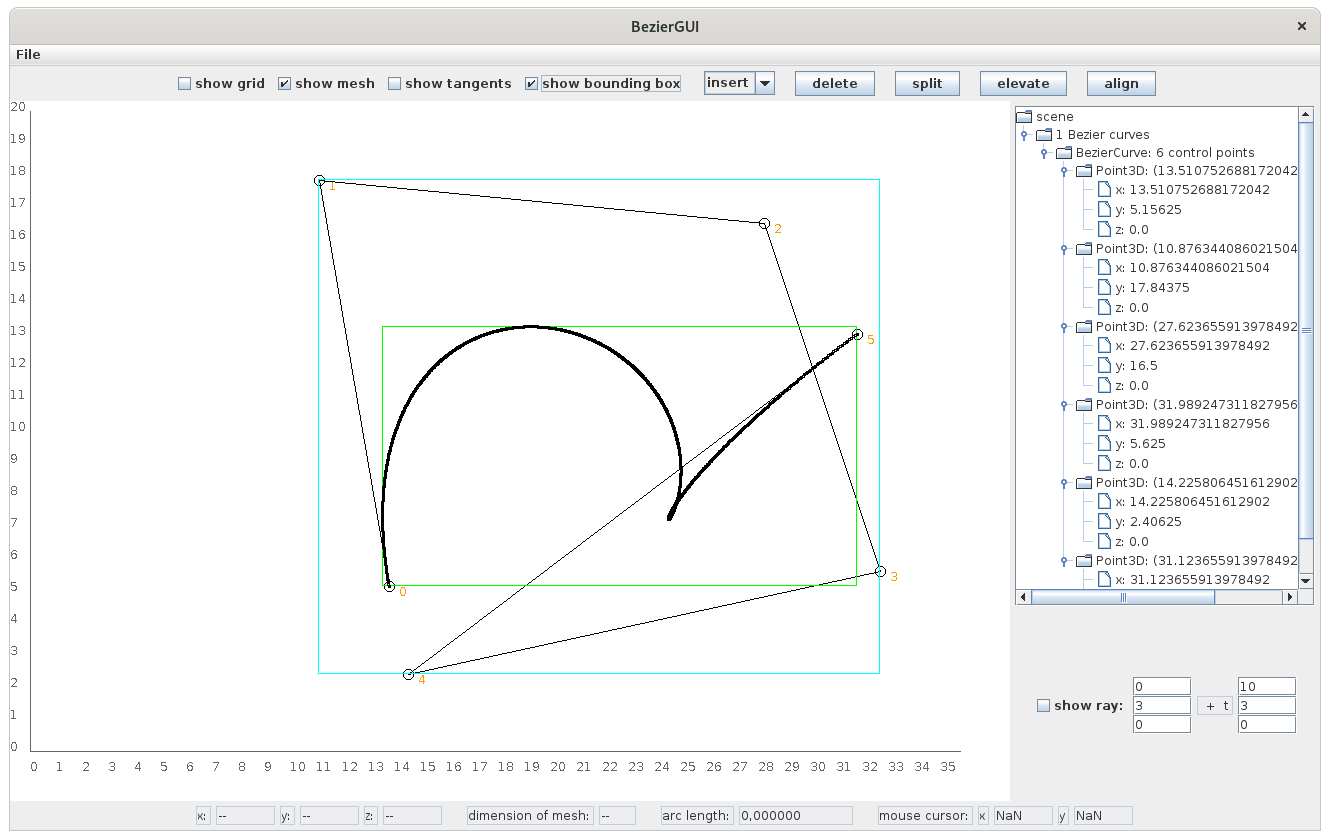
When the option show bounding box has been activated, axis-aligned bounding boxes will be drawn around the curves. Such axis-aligned bounding boxes are important tools for many algorithms in the field of computer graphics. I implemented two different approaches for the computation of bounding boxes. The first one simply spans an axis-aligned box around all participating control points, since the entire Bézier curve is contained within the convex hull of its control points. This characteristic is known as the convex hull property, and it represents a good and direct approximation for a bounding box. But, there is also the possibility of getting a bounding box that is much tighter in general. This approach uses the computation of the roots of some specific polynomials as a basis. Since (in the general case) the roots of polynomials of degree 5 and higher can only be obtained as an approximation by the application of numerical methods, I restricted myself to the computation of polynomials up to degree 4. Therefore, I only implemented this approach for Bézier curves with at most 6 control points. Whenever there is a Bézier curve with at least 7 control points, the tool will only display the bounding box that will be provided using the convex hull property.

As stated previously my main aim is to use Bézier objects for rendering purposes. Therefore, I implemented a method to calculate the intersection points between a given (3-dimensional) ray and the Bézier curve under consideration. This method uses the bounding box of the Bézier curve as an essential element. Each hit between the ray and the curve gets represented by red dots. The tool also displays the entrance, the exit and the middle between both along the ray within each bounding box. The discussed points are represented by small circles in the respective colors.

There exists the possibility to split a Bézier curve into two smaller pieces. The corresponding functionality can be triggered by using the button split. I implemented the curve splitting in a way such that it is possible to split the curve at any arbitrary double between 0 and 1. But, the GUI only supports splitting at the parameter 0.5 at the moment. So, the curve under consideration will be split exactly into two halves. Using this method another curve will be registered to the scene (this can be also seen in the scene graph on the right). Of course, all previously described operations can be applied to each curve registered to the scene.

Since I now have two curves registered to the scene, I can interact with both curves as I wish to. Therefore, I can also relocate a complete curve on the drawing canvas. And, as the next screen suggests, all previously mentioned tasks can be performed for each curve registered to the scene. Therefore, the drawing of the respective bounding boxes or the intersection functionality with a ray behaves as intended.

Finally, the File menu gives the possibility to store the control mesh for each curve, and also to restore previously saved meshes. This allows to interrupt the design process, and to continue the work later on.

Please let me know, if you are interested in playing around with the tool. I can provide a self-contained JAR for the described application.

NURBS

NURBS are a generalisation of Bézier curves where one can use the de Boor algorithm in order to evaluate a NURBS object. I also implemented a small application like the one presented in the previous section. But, for now I won't go into the details. Maybe some day (when I find the time) I will prepare a small introduction to this application.

All the previously presented tools have been developed in order to expand the applicability of my own private ray tracer 🤩. To be honest, I initially developed most of the tools long before the ray tracer (during my time at the Leipzig University). As an example, I have implemented a class named Polynomial which computes (among others) the roots of polynomials [1]. As it turns out, one needs to compute the roots of a quartic polynomial in order to determine the intersection of a ray with a torus. So, it is perfectly suitable to use the class Polynomial for the purpose of rendering a torus.

[1] Polynomials of degree 1 can be solved by a simple reorganisation of the equation. For polynomials of degree 2 we know the classical quadratic formula (p-q-formula). For cubic polynomials there exists the formula of Cardano, and for quartic polynomials we can use the solution given by Ferrari. For higher degrees there is no such formula in the general case (thanks to Galois).

But, anyways, it is pretty cool to exploit the interplay of those tools.

For now my ray tracer provides the following features:

• rendering of primitive objects (such as triangles, spheres, tori, disks, ...)
• rendering of freeform objects (like Bézier objects or NURBS objects)
• rendering of polygon-meshed objects described using the PLY standard
• rendering of textured objects
• sequential and parallel rendering
• space partitioning to reduce the computational overhead of the rendering process

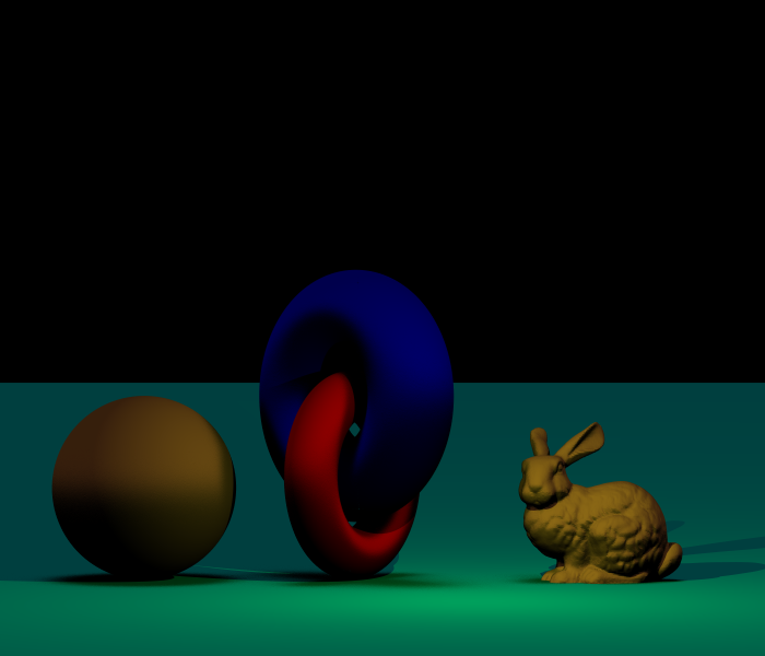
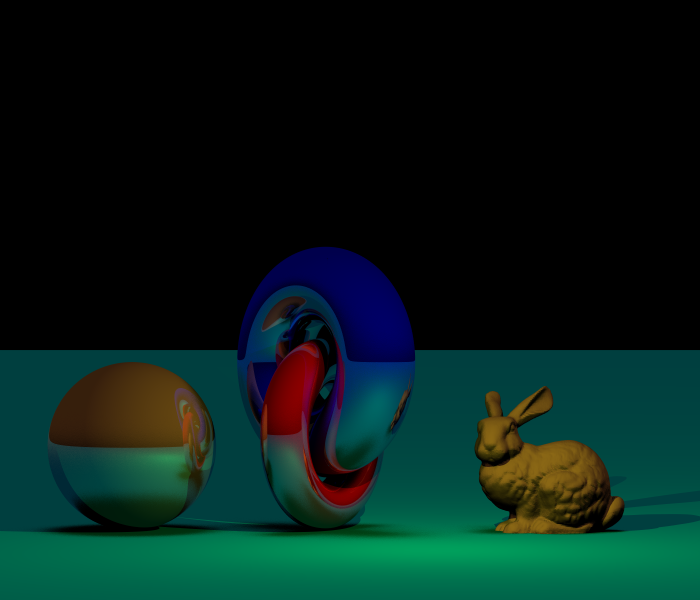
Below is a scene that has been rendered using my ray tracer. It shows a sphere, and two entangled tori right next to the famous Stanford bunny. A sphere and a torus are primitive objects in my application. I make use of the mentioned Polynomial library in order to calculate the intersection points between a torus and a ray. The bunny is given as a PLY model, and I directly use the files provided by Stanford University Computer Graphics Laboratory. One torus consists of a red reflective material, and the other of a blue reflective material. The sphere consists of a brown reflective material, whereas the bunny itself consists of a simple matte material. To reduce the aliasing effects of the pictures each scene was rendered using 128 samples per pixel.

The presentation starts by showing the scene with very restricted shading, meaning that the rendering simply results in a determination of the positioning of the objects within the scene. One can see the colored objects, but there is no influence of the shading of one object to another, or there is even no information about the illumination of the scene. Since there exists no shadow it is even impossible to clearly determine if the objects are placed on top of the plane, or if the objects are hanging in the air.

I want to discuss the scene in more detail now in order to describe some of the qualities that are typical for ray tracing.

One can specify the recursion depth for the calculation of reflected rays. This recursion depth determines the number of recursive rays that will be followed whenever a ray hits a reflective object. With a recursion depth of 1, the tracer computes only one hierarchy of reflected rays after a reflection occured. A recursion depth of 2 determines that the tracer computes another hierarchy of reflected rays for the rays that have been reflected in the first recursion step. This process continues until the maximal number of reflections has been reached. So, when the maximal recursion depth is 0, there is no reflection at all. Therefore, the tori are only rendered using their defined colors (blue and red), and the sphere is simply brown. For a maximal recursion depth of 1 one can see the reflection of the bunny on the blue torus, and the reflection of the tori on the sphere. Whereas the further increasing of the recursion depth only influences the reflections between the tori and the sphere.

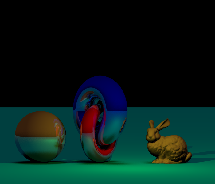
I rendered the scene using a constant ambience on the one hand, and oppose the results to ambient occlusion on the other hand. Ambient occlusion means that the ambient illumination of an object is directly determined by the objects surrounding it. Since the surrounding objects may block the light for the object, the shadows on a cornered object are more prominent than the shadows on an exposed object. This is the reason why the shadows on the tori appear sturdier. The lower half of the sphere appears darker because the light that could hit the lower half of the sphere is blocked by the plane, whereas there are no blocking objects for the upper half of the sphere. In contrast, the bunny is in principle brighter for the scene using ambient occlusion, since it is not so closely surrounded by other objects.

The described scene with constant ambience:

The same scene using ambient occlusion:

Since reflections are a strength of ray tracing (and since it is very nice to watch) you can find the same scene with a reflective underground (I took the scene with ambient occlusion and recursion depth 4):

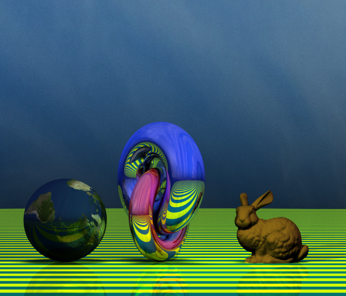
In order to shortly demonstrate the texture mapping abilities of my ray tracer, I mapped a simple procedural texture to the ground and a (rotated) picture of our precious planet to the sphere. I also mapped a picture of some clouds to the background in order to create the impression of a sky. Keep in mind that the textured sphere and the textured ground keep their reflective material. Therefore, the objects appear as a mixture of textures and reflections. The reflections of the various procedural stripes are nice to see on the surfaces of the different reflective objects, and the reflections of the sky are nice to see on the tori as well:

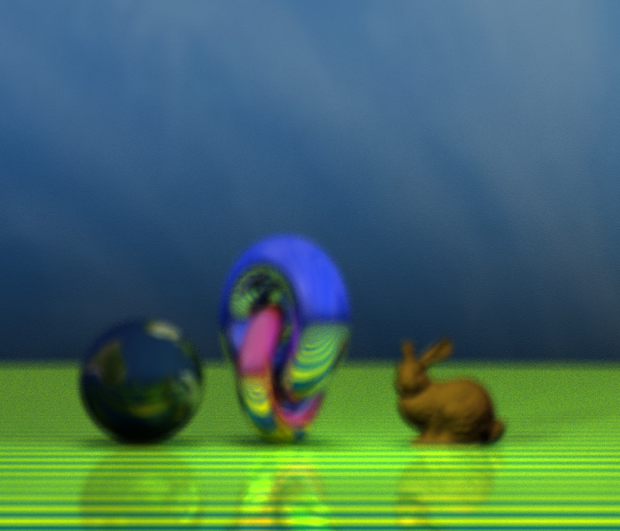
I as well integrated a thin lens camera making the whole scene appearing blurred:

To conclude this section, the next picture shows the scene where the tori now consist of a transparent material, giving the impression as if they were made from red or blue glass, respectively. Furthermore, the bunny has been manufactured from a reflective material:

I will further extend the software whenever I find the time to do so. For example, I plan to integrate constructive solid geometry in the near future, since this enables an even more flexible design for the objects.

Minesweeper

During my diploma studies I was once giving a talk where I had to understand and summarize a peer-reviewed and published paper from actual research. The aim of this presentation was to demonstrate that the student (it was me in this case) is able to understand and present a valuable contribution to a research topic. The mentioned talk was about the paper Minesweeper is NP-complete from Richard Kaye [2]. This paper demonstrates that one can become very rich when focussing on a solver for the game Minesweeper 🤑 (see P vs NP Problem and especially the rules there).

For the presentation of the talk I wanted to show drawings of the proposed Minesweeper configurations within my slides. Since it is very unlikely to get a desired configuration of the game area by starting a new game (using one of the standard implementations) over and over again, and since I did not want to draw the configurations with some photoshopping tool by hand, I finally decided to implement my own version of Minesweeper. This version had to support the integration of predefined configurations. And this is the story why I now own my personal implementation of the Minesweeper game. 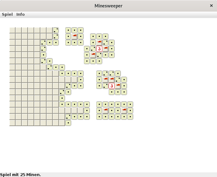The following slideshow represents a typical gameplay:

The slides of the mentioned talk can be found here (attention: language is German).

Please let me know, if you are interested in playing around with the tool. I can provide a self-contained JAR including all the sources.

[2] Besides this mentioned talk I also summarised the papers The equality problem for rational series with multiplicities in the tropical semiring is undecidable (from Daniel Krob) and Higher Dimensional Automata (from Zoltán Ésik and Zoltán L. Németh) during other courses. The GERMAN slides of my talk about the paper from Daniel Krob can be found here, and the slides of my talk about the paper from Ésik and Németh is here. Since those were my very first presentations at university, I did not even mention myself as the presenter of the slides. I only mentioned the authors of the referred papers (Krob, and Ésik / Németh resp.) instead 🤔.

Sudoku

I also implemented a primitive solver for the well-known Sudoku puzzles. This solver works by discarding all the numbers that are not possible for a specific cell (based on the environment of this cell). This process will be repeated until a valid solution for each cell has been found, or (if there is no unambiguous solution) until the possible solutions for each cell have not changed during an iteration of the algorithm. 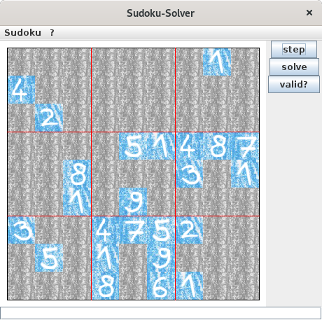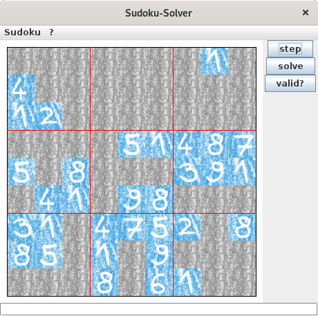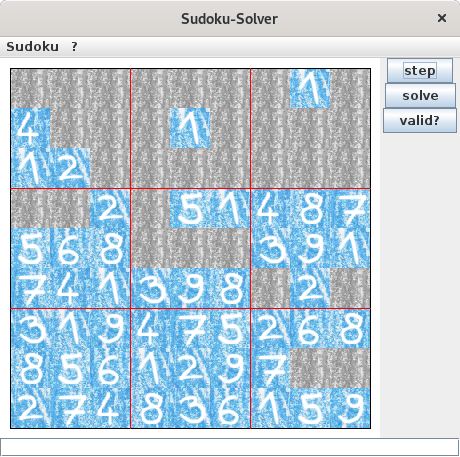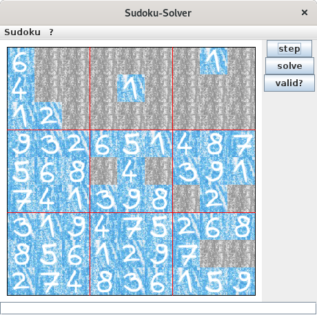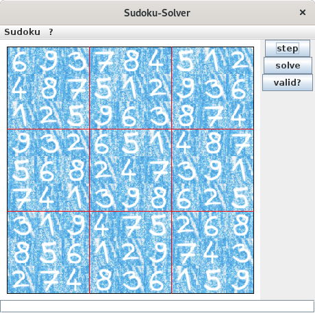The following slideshow represents the solving of a Sudoku. I have chosen the minimal [3] Sudoku presented at the German site of wikipedia for the show:

[3] The term minimal in this case states, that there need to be at least 17 predefined entries for the Sudoku under consideration. If there are fewer predefined entries it is not possible that there exists an unambiguous solution (see here for more details).